PostgreSQL pgvector混合搜索实战：向量相似度+全文关键词融合

PostgreSQL pgvector混合搜索实战：向量相似度+全文关键词融合 | 前端进阶之旅

Full translation

完整中文译文

我们真正在解决的搜索问题

如果你正在构建任何现代 AI 应用程序——无论是 RAG（检索增强生成）管道、语义搜索引擎，还是智能文档检索系统——你很可能遇到了一种根本性的矛盾：

向量相似性搜索能理解语义，但可能错过精确的关键词匹配。

全文搜索能捕捉精确术语，但无法理解语义关系。

如果两者可以兼得呢？

这正是混合搜索的承诺：将向量嵌入的语义理解与传统全文搜索的精确性相结合，全部在单一 PostgreSQL 数据库中，使用 pgvector 扩展实现。

在本综合指南中，我们将从头开始构建一个可用的混合搜索系统，分析其性能特征，并深入理解它为何有效——以及何时应该在你的 AI 工程项目中考虑实现它。

1. 为什么混合搜索对 AI 应用程序很重要 {#why-hybrid-search-matters}

RAG 革命及其检索问题

检索增强生成已成为构建需要访问外部知识的 AI 应用程序的主导范式。这个模式看似简单：

系统检索相关文档

LLM 使用检索到的上下文生成答案

第 2 步——检索——的质量往往决定了整个系统的成功。但这里有一个令人不安的事实：大多数 RAG 实现仅依赖向量相似性搜索，而这种方法存在明显的盲点。

向量搜索何时失效

考虑以下纯向量搜索表现不佳的场景：

全文搜索何时失效

传统全文搜索有互补的弱点：

混合搜索解决方案

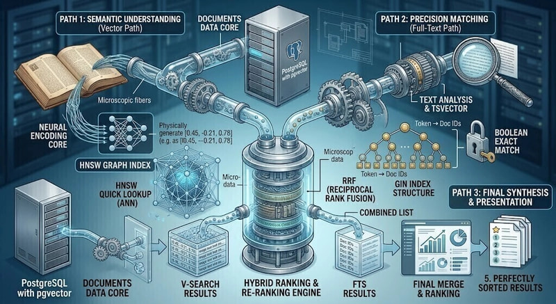
混合搜索结合了两种方法，使用互惠排名融合（Reciprocal Rank Fusion，RRF）等技术智能地合并结果。其结果是：更好的召回率、更好的精确率，以及对多样化查询类型更鲁棒的检索能力。

2. 理解搜索的两大支柱 {#understanding-the-two-pillars}

在深入实现之前，让我们为每种搜索方法建立一个清晰的 mental model。

向量相似性搜索

向量搜索将文本转换为高维嵌入——捕获语义含义的数值表示。相似的含义产生相似的向量，使以下成为可能：

语义匹配："happy" 能找到 "joyful"
概念搜索："how to fix a leak" 能找到 "plumbing repair guide"
跨语言检索：使用多语言模型，"hello" 能找到 "hola"

相似度通常用余弦距离来衡量，值越小表示相似度越高。

cosine_distance = 1 - cosine_similarity

PostgreSQL 的全文搜索使用：

分词（Tokenization）：将文本拆分为单词
规范化（Normalization）：词干提取（"running" → "run"）、小写化
停用词移除（Stop word removal）：消除常见词（"the"、"a"、"is"）
tsvector 创建：带位置的有序规范化词素列表
tsquery 匹配：对搜索词进行布尔运算

结果是基于词素的索引，能够实现快速、精确的关键词匹配。

互补性原理

这里有一个关键洞察：向量搜索和全文搜索以不同的方式失效。当你将它们结合时，一种方法的失败可以被另一种方法的成功所弥补。

                    ┌─────────────────┐
                    │   User Query    │
                    └────────┬────────┘
                             │
              ┌──────────────┴──────────────┐
              │                             │
              ▼                             ▼
    ┌─────────────────┐           ┌─────────────────┐
    │  Vector Search  │           │ Full-Text Search│
    │   (Semantic)    │           │   (Lexical)     │
    └────────┬────────┘           └────────┬────────┘
             │                             │
             │    ┌─────────────────┐      │
             └───►│  RRF Fusion     │◄─────┘
                  │  (Combining)    │
                  └────────┬────────┘
                           │
                           ▼
                  ┌─────────────────┐
                  │ Ranked Results  │
                  └─────────────────┘

3. 设置 PostgreSQL 环境 {#setting-up-postgresql}

要跟随本文操作，你需要：

PostgreSQL（建议 14+ 版本）
pgvector 扩展（v0.5+，我将使用 v0.7.4）
Python 3.8+ 以及以下包：psycopg（PostgreSQL 适配器）、pgvector（Python 集成）、faker（测试数据生成）、sentence_transformers（嵌入生成）

# Install pgvector (varies by platform)
# macOS with Homebrew:
brew install pgvector

# Ubuntu/Debian:
sudo apt install postgresql-15-pgvector

# From source:
git clone https://github.com/pgvector/pgvector.git
cd pgvector && make && make install

# Python dependencies
pip install psycopg[binary] pgvector faker sentence-transformers

让我们创建一个注重生产级就绪的 schema：

-- Enable the vector extension
CREATE EXTENSION IF NOT EXISTS vector;

-- Create the products table
CREATE TABLE products (
    id int GENERATED BY DEFAULT AS IDENTITY PRIMARY KEY,
    description text NOT NULL,
    embedding vector(384) NOT NULL
);

-- Create a helper function for RRF scoring
-- This will be used in our hybrid search query
CREATE OR REPLACE FUNCTION rrf_score(rank int, rrf_k int DEFAULT 50)
RETURNS numeric
LANGUAGE SQL
IMMUTABLE PARALLEL SAFE
AS $$
    SELECT COALESCE(1.0 / ($1 + $2), 0.0);
$$;

为什么是 384 维？multi-qa-MiniLM-L6-cos-v1 模型生成 384 维嵌入。这是一个平衡了以下因素的有意选择：

表达能力：足够的维度来捕获语义细微差别
存储效率：比 768 或 1536 维的替代方案更小
查询速度：距离计算更快

4. 构建数据集：从随机文本到嵌入 {#building-the-dataset}

数据生成策略

在本次演示中，我们将使用 Faker 生成合成数据，并使用句子转换器对其进行编码。虽然数据是人造的，但方法论是生产级可用的。

from faker import Faker
import psycopg
from pgvector.psycopg import register_vector
from sentence_transformers import SentenceTransformer

# Initialize Faker for synthetic data
fake = Faker()

# Generate 50,000 random sentences (50 words each)
# This simulates a product description corpus
sentences = [fake.sentence(nb_words=50) for _ in range(50_000)]

print(f"Generated {len(sentences)} sentences")
print(f"Sample: {sentences[0][:100]}...")

生成嵌入

# Load the sentence transformer model
# multi-qa-MiniLM-L6-cos-v1 is optimized for question-answering retrieval
model = SentenceTransformer('multi-qa-MiniLM-L6-cos-v1')

# Generate embeddings for all sentences
# This may take several minutes depending on your hardware
print("Generating embeddings...")
embeddings = model.encode(sentences, show_progress_bar=True)
print(f"Embedding shape: {embeddings.shape}")  # Should be (50000, 384)

加载数据到 PostgreSQL

# Connect to your database
# Replace with your actual connection details
conn = psycopg.connect(
    dbname="your_database",
    user="your_user",
    password="your_password",
    host="localhost",
    port="5432",
    autocommit=True
)

# Register the vector type with psycopg
register_vector(conn)

cur = conn.cursor()

# Use COPY for efficient bulk loading
with cur.copy("COPY products (description, embedding) FROM STDIN WITH (FORMAT BINARY)") as copy:
    copy.set_types(["text", "vector"])
    for content, embedding in zip(sentences, embeddings):
        copy.write_row((content, embedding))

print("Data loaded successfully!")
cur.close()
conn.close()

性能提示：COPY 命令比逐条 INSERT 语句在批量加载方面快几个数量级。对于 50,000 行，这种方法通常在几秒内完成，而不是几分钟。

5. 索引策略：GIN 和 HNSW 详解 {#indexing-strategy}

-- Full-text search index using GIN (Generalized Inverted Index)
CREATE INDEX products_description_gin_idx ON products
    USING GIN (to_tsvector('english', description));

## 深入解析：GIN 索引

对 `to_tsvector('english', description)` 的 GIN 索引值得仔细说明：

表达式索引：我们索引的不是原始的 description 列，而是 `to_tsvector()` 的输出。这意味着：

存储效率：不需要单独的 tsvector 列

自动一致性：索引始终与文本保持同步

查询优化：使用相同表达式的查询可以使用索引

为什么用 'english'？PostgreSQL 要求表达式索引中的函数是不可变的。由于带字典参数的 `to_tsvector()` 是不可变的（字典是固定的），我们必须显式指定它。这确保了：

索引构建和查询中的词干提取一致

不会因会话级配置变更而出现意外

## 深入解析：HNSW 索引

HNSW（Hierarchical Navigable Small World，分层可导航小世界）是一种基于图的近似最近邻搜索算法：

Layer 3 (最粗): A ─────────────────── B │ │ Layer 2: C ───┼─── D ─── E ──────── F │ │ │ │ │ Layer 1: G ───┼────┼────┼─────┼────H────┼─── I │ │ │ │ │ │ │ │ Layer 0 (最细): 所有向量都连接到最近的邻居


为什么 `ef_construction=256`？这会增加索引构建期间图结构的质量。权衡是更长的构建时间，但换来更好的查询性能和召回率。

## 6. 实现向量搜索 {#implementing-vector-search}

### 生成查询向量

```python
from sentence_transformers import SentenceTransformer

model = SentenceTransformer('multi-qa-MiniLM-L6-cos-v1')
query_embedding = model.encode('travel computer')

向量搜索查询

SELECT 
    id, 
    description, 
    rank() OVER (ORDER BY $1 <=> embedding) AS rank
FROM products
ORDER BY $1 <=> embedding
LIMIT 10;

理解这些操作符：

<=>：余弦距离操作符（0 = 完全相同，2 = 完全相反）

rank() OVER (ORDER BY ...)：窗口函数，根据距离分配排名

$1：嵌入向量的参数化查询占位符

  id   | description             | rank 
-------+-------------------------+-------
 10578 | ... travel ... computer |    1
 20763 | ... computer ...        |    2
 20894 | ... computer ...        |    3
   838 | Computer ...            |    4
 11045 | ...computer ...         |    5
 18548 | ... travel computer ... |    6  ← 排名应该更高！
 16564 | ... computer ...        |    7
 20402 | ...computer ...         |    8
 10346 | ... computer ...        |    9
 11243 | ... travel ... computer |   10

观察：记录 18548 包含精确短语 "travel computer"，但仅排第 6 位。这是纯向量搜索的根本局限——它优先考虑整体语义相似性，而不是精确短语匹配。

7. 实现全文搜索 {#implementing-full-text-search}

全文搜索查询

SELECT
    id,
    description,
    rank() OVER (
        ORDER BY ts_rank_cd(
            to_tsvector(description), 
            plainto_tsquery('travel computer')
        ) DESC
    ) AS rank
FROM products
WHERE
    plainto_tsquery('english', 'travel computer') @@ 
    to_tsvector('english', description)
ORDER BY rank
LIMIT 10;

解析查询

plainto_tsquery('english', 'travel computer')：将纯文本转换为 tsquery

结果：'travel' & 'comput'（词干化，AND 连接）

to_tsvector('english', description)：将文档转换为可搜索形式

结果：排序后的词干化标记数组，带位置信息

@@ 操作符：测试 tsquery 是否匹配 tsvector

ts_rank_cd()：覆盖密度排名

考虑搜索词的接近程度

词出现位置越接近分数越高

  id   | description                 | rank 
-------+-----------------------------+------
 18548 | ... travel computer ...     |    1  ← 正确！
  7372 | ... travel computer ...     |    1
 49374 | ... travel computer ...     |    1
 39214 | ... travel computer ...     |    1
 12875 | ... computer travel ...     |    1
  3712 | ... travel computer ...     |    1
 24719 | ... travel ... computer ... |    7  ← 词相隔较远
 31607 | ... travel ... computer ... |    7
 13674 | ... travel ... computer ... |    7
 42755 | ... computer ... travel ... |    7

观察：全文搜索正确地将 18548 识别为顶级结果，但它返回许多排名相同的结果。它缺乏区分整体语义相关性的能力。

8. 倒数排名融合（RRF）的妙用 {#rrf-explained}

倒数排名融合是一种排名聚合方法，将多个排名列表组合成单一排名。它由 Cormack 等人于 2009 年提出，现已成为信息检索的标准技术。

RRF_score(d) = Σ (1 / (k + rank_i(d)))

k = 平滑常数（通常为 50-60）

rank_i(d) = 文档 d 在结果列表 i 中的排名

规模无关：组合的是排名而非原始分数

向量距离和 ts_rank 分数具有不同的量纲

排名具有普遍的可比性

稳健：一个列表中的异常值不会主导结果

单个第 1 名贡献约 0.02

多个高排名会累积效果

简单：无需训练

不同于学习排序方法

确定性且可解释

PostgreSQL 实现

CREATE OR REPLACE FUNCTION rrf_score(rank int, rrf_k int DEFAULT 50)
RETURNS numeric
LANGUAGE SQL
IMMUTABLE PARALLEL SAFE
AS $$
    SELECT COALESCE(1.0 / ($1 + $2), 0.0);
$$;

为什么用 COALESCE？这可以优雅地处理 NULL 排名。如果一个文档只出现在一个结果列表中，它的「缺失」排名被视为对总和贡献 0。

为什么用 IMMUTABLE PARALLEL SAFE？

IMMUTABLE：相同输入总是产生相同输出（索引表达式必需）

PARALLEL SAFE：可以在并行工作线程中执行

分数分布分析

关键洞察：排名第 1 和排名第 40 之间的差异仅约 2 倍。这意味着同时出现在两个列表中比仅在其中一个列表中排名第 1 更有价值。

9. 构建混合搜索查询 {#constructing-hybrid-query}

SELECT
    searches.id,
    searches.description,
    sum(rrf_score(searches.rank)) AS score
FROM (
    -- 向量搜索子查询
    (
        SELECT
            id,
            description,
            rank() OVER (ORDER BY $1 <=> embedding) AS rank
        FROM products
        ORDER BY $1 <=> embedding
        LIMIT 40
    )
    UNION ALL
    -- 全文搜索子查询
    (
        SELECT
            id,
            description,
            rank() OVER (
                ORDER BY ts_rank_cd(
                    to_tsvector(description), 
                    plainto_tsquery('travel computer')
                ) DESC
            ) AS rank
        FROM products
        WHERE
            plainto_tsquery('english', 'travel computer') @@ 
            to_tsvector('english', description)
        ORDER BY rank
        LIMIT 40
    )
) searches
GROUP BY searches.id, searches.description
ORDER BY score DESC
LIMIT 10;

为什么每个子查询返回 40 个结果？

选择 40 是战略性的：

默认 hnsw.ef_search：PostgreSQL 的 HNSW 索引默认搜索 40 个候选

重叠可能性：需要 10 个最终结果，40 提供了 4 倍缓冲

性能平衡：结果越多融合效果越好，但查询越慢

混合搜索查询

┌─────────────────────────────────────────────────────────────┐
│                    Hybrid Search Query                       │
└─────────────────────────────────────────────────────────────┘
                              │
        ┌─────────────────────┴─────────────────────┐
        │                                           │
        ▼                                           ▼
┌───────────────────┐                   ┌───────────────────┐
│  Vector Search    │                   │  Full-Text Search │
│  (HNSW Index)     │                   │  (GIN Index)      │
│                   │                   │                   │
│  Returns 40 rows  │                   │  Returns 40 rows  │
│  with ranks 1-40  │                   │  with ranks 1-40  │
└─────────┬─────────┘                   └─────────┬─────────┘
          │                                       │
          └───────────────┬───────────────────────┘
                          │
                          ▼
              ┌───────────────────────┐
              │    UNION ALL          │
              │  (80 rows total)      │
              └───────────┬───────────┘
                          │
                          ▼
              ┌───────────────────────┐
              │   GROUP BY id         │
              │   SUM(rrf_score(rank))│
              └───────────┬───────────┘
                          │
                          ▼
              ┌───────────────────────┐
              │   ORDER BY score DESC │
              │   LIMIT 10            │
              └───────────────────────┘

混合搜索示例结果

  id   | description                 |         score          
-------+-----------------------------+------------------------
 18548 | ... travel computer ...     | 0.03746498599439775910  ← Top!
  7372 | ... travel computer ...     | 0.01960784313725490196
 12875 | ... computer travel ...     | 0.01960784313725490196
 10578 | ... travel ... computer ... | 0.01960784313725490196
 39214 | ... travel computer ...     | 0.01960784313725490196
 49374 | ... travel computer ...     | 0.01960784313725490196
  3712 | ... travel computer ...     | 0.01960784313725490196
 20763 | ... computer ...            | 0.01923076923076923077
 20894 | ... computer ...            | 0.01886792452830188679
   838 | Computer ...                | 0.01851851851851851852

记录 18548（"正确答案"）：

同时出现在两个结果列表中

向量排名：6 → RRF 贡献值：1/(50+6) = 0.0179

全文搜索排名：1 → RRF 贡献值：1/(50+1) = 0.0196

记录 7372、12875 等：

在全文搜索中出现，排名为 1（或并列）

在向量搜索中出现，排名较低

综合得分：约 0.0196

记录 20763、20894、838：

仅在向量搜索中出现（排名较高）

关键洞察：记录 18548 同时出现在两个列表中且排名靠前，使其综合得分提升至第一名，验证了混合搜索方法的有效性。

10. 使用 EXPLAIN ANALYZE 进行性能分析 {#performance-analysis}

EXPLAIN ANALYZE
SELECT ...;  -- Our hybrid search query

Limit  (cost=789.66..789.69 rows=10 width=365) (actual time=8.516..8.519 rows=10 loops=1)
  ->  Sort  (cost=789.66..789.86 rows=80 width=365) (actual time=8.515..8.518 rows=10 loops=1)
        Sort Key: (sum(COALESCE((1.0 / (("*SELECT* 1".rank + 50))::numeric), 0.0))) DESC
        Sort Method: top-N heapsort  Memory: 32kB
        ->  GroupAggregate  (cost=785.53..787.93 rows=80 width=365) (actual time=8.435..8.495 rows=79 loops=1)
              Group Key: "*SELECT* 1".id, "*SELECT* 1".description
              ->  Sort  (cost=785.53..785.73 rows=80 width=341) (actual time=8.430..8.436 rows=80 loops=1)
                    ->  Append  (cost=84.60..783.00 rows=80 width=341) (actual time=0.877..8.414 rows=80 loops=1)
                          ->  Subquery Scan on "*SELECT* 1"  
                                ->  Limit  
                                      ->  WindowAgg  
                                            ->  Index Scan using products_embeddings_hnsw_idx on products  
                                                  Order By: (embedding <=> '<redacted>'::vector)
                          ->  Subquery Scan on "*SELECT* 2"  
                                ->  Limit  
                                      ->  Sort  
                                            ->  WindowAgg  
                                                  ->  Sort  
                                                        ->  Bitmap Heap Scan on products products_1  
                                                              Recheck Cond: ('''travel'' & ''comput'''::tsquery @@ ...)
                                                              ->  Bitmap Index Scan on products_description_gin_idx  
                                                                    Index Cond: (to_tsvector('english'::regconfig, description) @@ ...)

Planning Time: 0.193 ms
Execution Time: 8.553 ms

性能分解

索引使用确认

执行计划确认两个索引均被利用：

Index Scan using products_embeddings_hnsw_idx — HNSW 向量索引

Bitmap Index Scan on products_description_gin_idx — GIN 全文索引

扩展性考量

对于数百万行级别的生产工作负载：

11. 生产环境考量与权衡 {#production-considerations}

何时使用混合搜索

-- 查询时参数（值越高 = 召回率越好，速度越慢）
SET hnsw.ef_search = 100;

-- 索引时参数（需要重建索引）
-- m: 每个节点的连接数（默认 16）
-- ef_construction: 构建期间的候选列表大小（默认 64）

-- 使用不同的词典
to_tsvector('simple', description)  -- 无词干提取
to_tsvector('english', description) -- 英语词干提取

-- 针对领域特定术语的自定义词典
CREATE TEXT SEARCH DICTIONARY custom_dict (...);

-- k=50（默认）：平衡
-- k=10：更偏重排名靠前的结果
-- k=100：更平缓的分数分布

SELECT sum(rrf_score(rank, 10)) AS score  -- 更激进的策略

混合搜索 vs. 替代方案

12. 下一步与未来研究方向 {#next-steps}

立即可做的改进

添加重排序：使用跨编码器模型对顶部结果进行重排序

查询扩展：在搜索前使用同义词扩展查询

元数据过滤：与结构化过滤器结合

缓存：缓存频繁查询的向量

在真实数据集上基准测试：测量 recall@k 的提升

比较 FTS 算法：ts_rank vs ts_rank_cd vs 自定义

优化 RRF 参数：网格搜索最优 k 值

多向量方法：ColBERT 风格的晚交互

生产部署清单

□ 设置连接池（PgBouncer）
□ 配置 maintenance_work_mem 用于索引构建
□ 设置查询延迟监控
□ 实现查询