从个人生产力到组织能力：龙Suite-Pilot 与 SLS 的 AI 编码度量实践

本文详细介绍了使用 LoongSuite-Pilot 和阿里云 SLS 度量、分析和优化组织 AI 编码智能体使用情况及 ROI 的工程方法。

引言：编码变快了，但为什么组织没有跟上？

2026 年 5 月，Google Cloud DORA 团队发布了《AI 辅助软件开发的 ROI》。与前一年专注于个人采用率的《DORA 2025 年度 DevOps 状态报告》不同，该报告直接针对组织层面的问题：

"问题不再是 AI 辅助开发是否有效——而是如何向业务证明它有效。"

报告提供了一组模型数据。以 500 人的工程团队为例，AI 工具年度投资约 840 万美元，预期回报 1160 万美元，首年 ROI 约 39%。然而，这种回报并非自动实现。DORA 明确指出，编码速度的提升不会自动转化为组织产出：

"编码速度的初步提升很有前景，但并不会自动转化为底线收益。"

报告引入 J 曲线（先降后升的曲线）概念来解释这一机制。团队在采用 AI 工具的早期会经历生产力下降期。流程适配、习惯切换和提示词调优都是学习成本。只有在团队越过低谷并将恢复的能力重新投入到减少返工而非直接裁员时，ROI 才会在曲线的后期实现。同时，DORA 延续了 2025 年报告的核心判断：

"AI 是一个放大器，而非变革者。它放大了优势和 dysfunction。"

数据显示，AI 在全新（greenfield）项目中可带来 35% 至 40% 的效率提升，但在遗留代码上不足 10%。如此大的差异意味着，同一公司内不同团队的回报曲线可能完全不同。没有事件级度量能力的组织甚至无法判断自身 J 曲线走到了哪里。

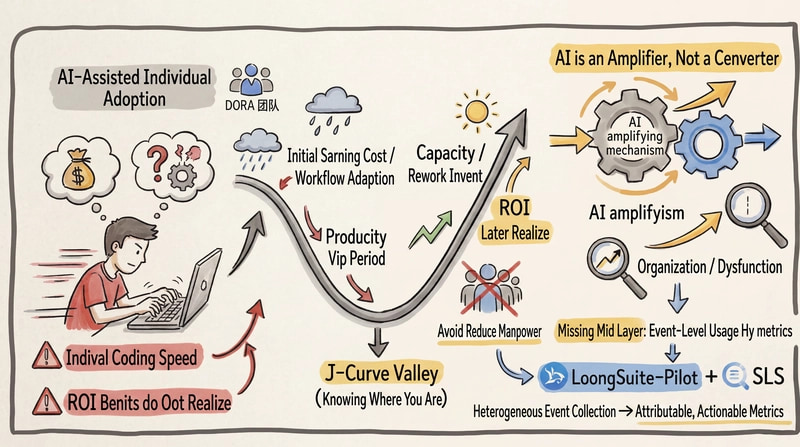
这正是大多数当前研发组织面临的困境：手中只有两类数据。一类是个人自报的满意度问卷（主观且不可追溯），另一类是 CI/CD 流水线的聚合 KPI（告诉你是什么，但不解释为什么）。真正缺失的是中间层：能下钻到智能体、模型、技能或部门的、事件级的 AI 编码使用行为度量。这使得组织能够准确回答：J 曲线走到了哪里、哪些团队已进入曲线后期、哪些仍在低谷。

本话题介绍的 LoongSuite-Pilot × 阿里云日志服务（SLS）集成，正是这个度量层的工程实现。LoongSuite-Pilot 按照龙Suite GenAI 语义规范（阿里云基于 OpenTelemetry GenAI 语义约定推出的扩展规范）统一采集异构智能体的事件流。SLS 仪表盘将事件解读为组织级度量，支持下钻、归因和行动。

数据接入层：从采集到 SLS 落地

在构建度量仪表盘之前，先来解决数据从何而来的问题。

我们选择度量的不是提交了多少行代码或合并了多少个 Pull Request（PR），而是 AI 编码智能体本身的使用行为：谁使用了哪个智能体、选择了哪个模型、消耗了多少 tokens、调用了哪些工具和技能。

数据模型采用经典的事实表与维度表分离设计。两张表通过 user.id 和 work_no 关联。事实表与维度表的分离使得度量层可以通过 JOIN 灵活叠加组织维度，无需在事件上报时嵌入组织信息。

事件事实表：AI 编码智能体的行为日志

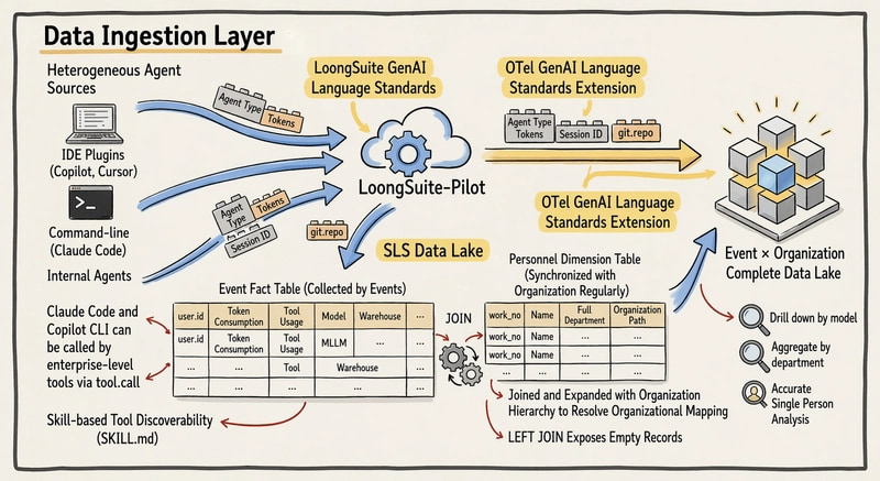
事实表是整个度量仪表盘的核心数据源。每条记录对应一次智能体调用事件。核心字段包括：

• 用户标识：user.id
• 会话：gen_ai.session.id
• 智能体 / Provider / 模型：gen_ai.agent.type、gen_ai.provider.name、gen_ai.request.model、gen_ai.response.model
• Token 消耗：gen_ai.usage.input_tokens、gen_ai.usage.output_tokens、gen_ai.usage.total_tokens
• 工具调用：gen_ai.tool.name、gen_ai.tool.call.arguments.file_path、event.name

这些字段与龙Suite GenAI 语义规范对齐。OpenTelemetry GenAI 语义约定被业界公认为起点。然而，社区标准天然需要平衡广泛适用性和长期稳定性，目前仍处于发展状态。在实际业务中，AI 智能体的调用链往往比"单一用户 × 单一模型"要复杂得多。一个请求可能跨越多个智能体的协同调用。

龙Suite GenAI 语义规范正是基于大量实践场景，对 OpenTelemetry 社区标准的扩展规范。该规范现已开源，优化能力未来将逐步贡献回社区上游。与此规范对齐的直接好处是，Claude Code、Copilot、Cursor、Qoder 以及各类内部智能体的上报指标天然一致，无需事后进行字段对账。

这些事件通过 LoongSuite-Pilot 统一采集。LoongSuite-Pilot 不区分智能体来源和 IDE 形态。无论是命令行形式的 Claude Code 还是 IDE 插件形式的 Copilot 或 Cursor，都落入同一张事实表。采集粒度为事件级。每次智能体调用、每次工具调用、每次 token 消耗均作为独立事件上报，而非按会话聚合后再上报。

事件级粒度带来三方面的工程价值：

第一，异构智能体的可比性：同一 token 下 Claude Code 和 Copilot 的统计指标完全一致，跨工具比较和聚合无需任何指标转换。

第二，会话级可追溯性：通过 gen_ai.session.id 下钻到单次 tool.call，故障排查可以精确到"本次会话中第三次工具调用传入了什么参数"，而非停留在"这个人上周 token 消耗较高"。

第三，技能和工具的可观测性：gen_ai.tool.call.arguments.file_path 将工具调用与具体的 SKILL.md 文件路径关联，使"团队积累的技能是否真正被使用"成为一个可量化的问题。

人员维度表：组织关系映射

事件流解决"发生了什么"，人员维度表解决"是谁在做的"。事件中的用户标识映射到组织拓扑，从而支持按部门、团队、人员下钻度量。维度表定期同步到 SLS。核心字段包括 work_no（员工工号）、show_name（姓名）、dept_name（完整部门路径，例如"技术研发部-工程平台部-数据服务组"）。

为什么必须将组织关系作为独立维度表集成，而非在事件上报时注入部门信息？原因有三：

第一，解耦。人员维度表随组织调整持续更新，而事件一旦上报就不应被追溯修改。只有维度表独立，才能"基于最新组织结构查看历史数据"。

第二，LEFT JOIN 暴露空白。通过 LEFT JOIN + WHERE user_id IS NULL，可以直接列出_dimension 表有记录但事件表无记录的人员——即"已注册但未上报"的人。这个"已注册但未上报"名单往往比所有酷炫图表更能推动落地。

Third, level splitting is completed at one time. The department path is split by level into three layers: tier-1 department, tier-2 department, and team. All downstream charts only need to JOIN the dimension table to obtain the complete organization dimension. You do not need to repeat the splitting logic for each graph.

第三，层级拆分一次完成。部门路径按层级拆分为三个层级：一级部门、二级部门和团队。所有下游图表只需 JOIN 维度表即可获得完整的组织维度，无需在每个图表中重复拆分逻辑。

The core questions answered by the data integration layer boil down to three: what to collect (LoongSuite GenAI semantics events), how to collect (uniform collection by LoongSuite-Pilot), and who to associate with (personnel dimension table). After the three steps are completed, SLS has a complete data foundation of "event × organization."

数据集成层要回答的核心问题归根结底只有三个：收集什么（LoongSuite GenAI 语义事件）、如何收集（通过 LoongSuite-Pilot 统一采集）、与谁关联（人员维度表）。完成这三步后，SLS 就拥有了"事件 × 组织"的完整数据基础。

Measure Layer: from a Public CTE to an Actionable AI Coding Agent Measure Dashboard

度量层：从公共 CTE 到可操作的 AI 智能体度量仪表盘

Why Choosing the SLS Dashboard as the Analysis Layer?

为什么选择 SLS 仪表盘作为分析层？

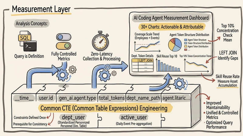
After having the data foundation, the next step is to choose an analysis carrier. We directly build the entire measure dashboard on the SLS dashboard using SQL. The core reason for choosing this path is flexibility. AI coding measure is a scenario where the metric highly varies by team and requirements undergo fast iteration. The analysis layer must give users sufficient freedom.

有了数据基础后，下一步是选择分析载体。我们直接使用 SQL 在 SLS 仪表盘上构建整套度量仪表盘。选择这条路径的核心原因是灵活性。AI 编码度量是一个指标因团队而异且需求迭代迅速的场景，分析层必须给用户足够的自由度。

First, query is definition. Behind each chart on an SLS dashboard is an SQL statement. If requirements change, you can modify the SQL statement to make the changes take effect immediately. You do not need to wait for the product to be published or for configuration support.

第一，查询即定义。SLS 仪表盘上每个图表背后都是一条 SQL 语句。如果需求变更，可以直接修改 SQL 语句使变更立即生效，无需等待产品发布或配置支持。

Second, definitions are fully self-controlled. "What counts as an active user", "how to break down departments", and "whether the denominator for the coverage rate is registered employees or all employees" — these definition choices vary by organization and have no ground truth. SLS SQL allows each team to flexibly define them based on their own business characteristics. Your organization can break down by level-3 departments, while mine breaks down by project groups. Your definition of active is "having events in the past 7 days", while mine is "having events in the past 30 days and Tokens > 1000". These differences can be expressed by a single WHERE clause at the SQL layer.

第二，定义完全自主可控。"什么算活跃用户"、"如何拆分部门"、"覆盖率的分母是注册员工还是全体员工"——这些定义选择因组织而异，没有标准答案。SLS SQL 允许每个团队根据自身业务特点灵活定义。你的组织可以按三级部门拆分，我的按项目组拆分。你对活跃的定义是"过去 7 天有事件"，我的是"过去 30 天有事件且 Tokens > 1000"。这些差异只需在 SQL 层用一个 WHERE 子句即可表达。

Third, collection and analysis are on the same platform. After events are delivered to SLS, they can be queried immediately. There is no additional extract, transform, and load (ETL) link or T+1 delay. For example, if you just connect a new Agent, you can confirm whether data flows in normally on the dashboard within a few minutes after it is published. The verification closed loop is extremely short.

第三，采集与分析在同一平台。事件投递到 SLS 后即可立即查询，没有额外的 ETL 链路或 T+1 延迟。例如，刚接入一个新的 AI 智能体，在其发布后几分钟内就能在仪表盘上确认数据是否正常流入。验证闭环极短。

After flexibility is established, the next question is: How to maintain definition consistency across 30+ charts?

在灵活性确立之后，下一个问题是：如何在 30+ 个图表间保持定义一致性？

CTE: the Engineering Skeleton of a Report

CTE：报表的工程骨架

Flexibility solves the problem of "whether it can be modified". However, if each chart on a dashboard with 30+ charts has its own SQL statement, definition inconsistencies and maintenance costs will quickly spiral out of control. Therefore, the engineering core lies in the design of the analysis hierarchy: from metric definition, to pre-aggregation, to dimension progression, and then to specific charts, each layer serves the next layer.

灵活性解决的是"能否修改"的问题。然而，如果一个包含 30+ 图表的仪表盘中每个图表都有独立的 SQL 语句，定义不一致和维护成本将很快失控。因此，工程核心在于分析层级的设计：从指标定义，到预聚合，到维度递进，再到具体图表，每一层都为下一层服务。

All charts on the entire dashboard share the same group of CTE. This is not an SQL trick, but the engineering prerequisite for the entire report to achieve "definition consistency, maintainability, and controllable performance".

整个仪表盘上所有图表共享同一组 CTE。这不是 SQL 技巧，而是整份报表实现"定义一致、可维护、性能可控"的工程前提。

CTE 1: dept_user (Standardization of Personnel Dimension Table)

CTE 1：dept_user（人员维度表标准化）

WITH dept_user AS (
SELECT
work_no,
show_name,
COALESCE(SPLIT_PART(dept_name, '-', 1), '') AS dept_name_1, -- Level-1 department, such as "Technology R&D Department"
COALESCE(SPLIT_PART(dept_name, '-', 2), '') AS dept_name_2, -- Level-2 department, such as "Engineering Platform Department"
COALESCE(SPLIT_PART(dept_name, '-', 3), '') AS dept_name_3 -- Team, such as "Data Service group"
FROM <dept-logstore>
GROUP BY work_no, show_name, dept_name
)

The core of this CTE is to break down the complete department path (such as Technology R&D Department-Engineering Platform Department-Data Service group) into a three-level hierarchy (level-1 department/level-2 department/team). The definition constraint of "statistics scope" is defined only once here. All downstream charts automatically inherit it through JOIN.

这个 CTE 的核心是将完整的部门路径（如"技术研发部-工程平台部-数据服务组"）拆分为三级层级（一级部门/二级部门/团队）。"统计范围"的定义约束只在这里定义一次，所有下游图表通过 JOIN 自动继承。

CTE 2: active_user (Event Pre-aggregation)

CTE 2：active_user（事件预聚合）

active_user AS (
 SELECT
 date_trunc('day', __time__) AS t,
 "user.id" AS user_id,
 coalesce(nullif("gen_ai.agent.type", 'null'), 'unknown') AS agent_type,
 coalesce(nullif("gen_ai.provider.name", 'null'), 'unknown') AS provider,
 coalesce(nullif("gen_ai.request.model", 'null'),
 nullif("gen_ai.response.model", 'null'), 'unknown') AS model,
 sum(coalesce("gen_ai.usage.input_tokens", 0)) AS input_tokens,
 sum(coalesce("gen_ai.usage.output_tokens", 0)) AS output_tokens,
 sum(coalesce("gen_ai.usage.total_tokens", 0)) AS total_tokens,
 count(1) AS events
 FROM <events-logstore>
 GROUP BY t, user_id, agent_type, provider, model
)

This CTE performs five-dimension pre-aggregation by day × user × Agent × supplier × model to produce the number of Tokens and events. The key benefit of pre-aggregation is: The vast majority of charts directly reuse active_user JOIN dept_user, and you do not need to repeatedly write aggregation logic for each chart.

该 CTE 按天 × 用户 × AI 智能体 × 供应商 × 模型五个维度进行预聚合，生成 Tokens 数量和事件数。预聚合的关键好处是：绝大多数图表直接复用 active_user JOIN dept_user，无需在每个图表中重复编写聚合逻辑。

Convention for JOIN between two tables:

两张表之间的 JOIN 约定：

FROM dept_user d
JOIN active_user a ON d.work_no = a.user_id

The design quality of the CTE layer determines three fundamentals of the entire dashboard: definition consistency (constraints are defined only once), maintainability (modifying one CTE automatically takes effect for all charts), and query performance (pre-aggregation reduces the scan volume of downstream SQL statements). For the 8 sections detailed later, the vast majority directly reuse CTE as the data source. A small number of charts that require finer granularity (such as Skill path fetch and repository dimension aggregation) revert to the original event table for separate queries. However, even so, the JOIN logic of the personnel dimension table still reuses dept_user to maintain definition consistency.

CTE 层的设计质量决定了整个仪表盘的三个基础：定义一致性（约束只定义一次）、可维护性（修改一个 CTE 自动对所有图表生效）、查询性能（预聚合减少下游 SQL 的扫描量）。对于后面详述的 8 个板块，绝大多数直接复用 CTE 作为数据源。少量需要更细粒度的图表（如 Skill 路径获取和仓库维度聚合）会回退到原始事件表进行单独查询。但即便如此，人员维度表的 JOIN 逻辑仍然复用 dept_user 以保持定义一致性。

Analysis Dimension Progression The 8 sections of the measure dashboard are not randomly stacked charts, but are designed progressively according to the analysis hierarchy:

分析维度递进 度量仪表盘的 8 个板块并非随机堆叠的图表，而是按照分析层级递进设计的：

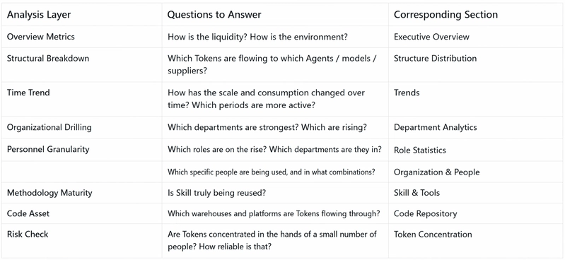
From "overall perception" to "structure breakdown" and then to "threat validation", each layer provides context for finer-granularity analysis.

从"整体感知"到"结构拆解"再到"威胁验证"，每一层都为更细粒度的分析提供上下文。

The data in the following screenshots is all analog data, which is used to illustrate the report structure and analysis logic, and does not represent real business data.

以下截图中的数据均为模拟数据，仅用于说明报表结构和分析逻辑，不代表真实业务数据。

A row of comparison cards at the top serves as the 'water level gauge' for the entire dashboard: active employees, total tokens, session count, Agent events, tokens per capita, and employees without reported usage. Each card includes a week-over-week (WoW) comparison against the same period last week. Together, these cards elevate the question of "how much is being used" from individual perception to the organizational level—revealing how many people are actively using it and whether overall usage this week is trending up or down compared to last week.

顶部的一排对比卡片充当整个仪表盘的"水位计"：活跃员工数、Total Tokens、会话数、AI 智能体事件数、人均 Tokens 和无报备使用的员工数。每张卡片都包含与上周同期的环比（WoW）对比。这些卡片共同将"用了多少"的问题从个人感知提升到组织层面——揭示有多少人在积极使用，以及本周整体用量相比上周是上升还是下降。

Cards showing abnormal week-over-week changes serve as drill-down entry points: if a metric drops, you can navigate to the corresponding section to identify the root cause. This shifts management decisions from intuition-driven to evidence-based.

显示环比异常变化的卡片作为下钻入口：如果某个指标下降，可以导航到相应板块找出根本原因。这将管理决策从凭感觉驱动转变为基于证据驱动。

To ensure WoW figures are reliable, the WoW calculation needs to work around a common pitfall: compare() is not compatible with cross-table CTE joins, and will throw an error directly. To address this, the calculation is instead implemented using manual windowing:

为确保 WoW 数据可靠，WoW 计算需要规避一个常见陷阱：compare() 不兼容跨表 CTE JOIN，会直接报错。为此，计算改用手动窗口实现：

time_base AS (
  SELECT max(__time__) AS t_max FROM <event table>
),
cur_agg AS (
  SELECT "user.id" AS user_id, count(*) AS events
  FROM <event table>
  WHERE __time__ >= (SELECT t_max - 604800 FROM time_base)
  GROUP BY "user.id"
),
prev_agg AS (
  SELECT "user.id" AS user_id, count(*) AS events
  FROM <event table>
  WHERE __time__ >= (SELECT t_max - 1209600 FROM time_base)
    AND __time__ < (SELECT t_max - 604800 FROM time_base)
  GROUP BY "user.id"
)
-- JOIN dept_user separately and compute the WoW comparison after aggregation
SELECT
  cur.cnt AS "Current value",
  CASE WHEN prev.cnt > 0
       THEN round((1.0 × cur.cnt / prev.cnt - 1) × 100, 2)
  END AS "Compared to last week (%)"
FROM cur, prev

The SQL is longer, but it's the only reliably stable syntax under the "CTE + JOIN" architecture.

SQL 更长，但在"CTE + JOIN"架构下这是唯一可靠稳定的语法。

Section 2: Structure Distribution

第 2 板块：结构分布

三个饼图分别按 AI Agent 类型、模型和供应商划分 Token 占比，回答了组织层面的资源配置问题：哪个 AI 智能体在使用上领先，Token 是集中在一个供应商还是分散在多个供应商，团队的主要模型是什么。这些答案直接决定了工具是否需要整合、如何集中采购供应商、以及如何聚合成本。

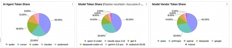
得益于 CTE 基座，获取这些决策所需的数据变得非常轻量：三个图表都运行在 dept_user JOIN active_user 上，唯一的区别只是 GROUP BY 的字段不同：

SELECT
  a.agent_type AS "AI Agent",
  sum(a.total_tokens) AS "Total tokens"
FROM dept_user d
JOIN active_user a ON d.work_no = a.user_id
GROUP BY a.agent_type
ORDER BY "Total tokens" DESC

预聚合使每个图表只需关注自身的 GROUP BY 维度，而切换模型或供应商版本只需要改动一个字段。

趋势图将"当前状态"延伸到"趋势"：覆盖人数趋势（员工数和事件数双线）、Token 消耗趋势（输入/输出/总量三条线）、各 AI 智能体的事件和 Token 趋势（按 agent_type 分组）以及 Token 使用时段分布。

只有从趋势中才能判断 AI 工具的使用规模是稳步增长还是在一波推广后退潮，以及某个 AI 智能体是越来越重要还是逐渐被替代。时段分布提供了工作节奏的画像。如果 Token 集中在清晨，说明 AI 自动化作业的比例在上升。这与工作时间人工交互驱动的使用模式完全不同，对应的管理动作也应该不同。

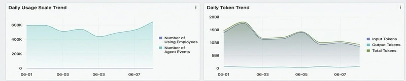
大多数折线图可以直接复用 day 粒度的 GROUP BY a.t active_user。但时段分布是个例外。active_user 已经过 date_trunc('day', __time__) 处理，小时维度已被丢弃。要还原小时分布，必须绕过 CTE，从一个新的 hourly_user 开始独立聚合：

hourly_user AS (
  SELECT
    date_format(__time__, '%H:00') AS h,
    "user.id" AS user_id,
    sum(coalesce("gen_ai.usage.total_tokens", 0)) AS total_tokens
  FROM < event table>
  GROUP BY h, user_id
)
SELECT a.h AS t, sum(a.total_tokens) AS "tokens"
FROM dept_user d
JOIN hourly_user a ON d.work_no = a.user_id
GROUP BY a.h
ORDER BY t

这是下游图表需要比 CTE 更细粒度时的典型回退路径。

第四部分：部门统计

部门统计将视角从个人切换到团队。部门 Token 事实表（部门、总人数、用户数、覆盖率%、事件数、输入/输出/总量 Token、人均 Token）与"未正常上传统计数据的员工列表"配对。然后叠加 Top 10 横向条形图，分别按总量 Token、覆盖率、人均 Token 排序。

三个维度指向三种不同行动：规模小的部门需要推广，覆盖率低的部门需要从"个人早期采用"进阶到"团队标准化"，人均使用量低的部门可能需要优化工具配置或改进使用方法。

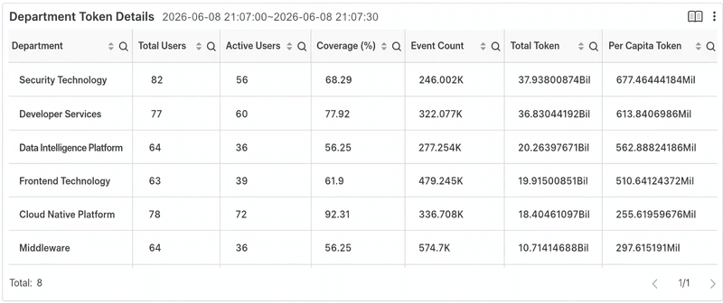
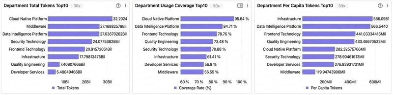
要让这些排名有意义，"用户数为 0"的部门不能被过滤掉，因为它们恰恰就是推广的目标。因此事实表使用 LEFT JOIN 而不是 INNER JOIN：

SELECT
  d.dept_name_2 AS "Department",
  approx_distinct(d.work_no) AS "Total number of people",
  approx_distinct(a.user_id) AS "Number of users",
  round(100.0 × approx_distinct(a.user_id) / nullif(approx_distinct(d.work_no), 0), 2) AS "Coverage rate (%)",
  sum(a.total_tokens) AS "Total Tokens",
  round(1.0 × sum(a.total_tokens) / nullif(approx_distinct(a.user_id), 0), 2) AS "Tokens per capita"
FROM dept_user d
LEFT JOIN active_user a ON d.work_no = a.user_id
GROUP BY d.dept_name_2
ORDER BY "Total Tokens" DESC

LEFT JOIN 使得"用户数为 0"的部门得以保留在表中。这些部门不会被 INNER JOIN 默默过滤掉。"未上报"列表同样基于这个 JOIN，只需加上 WHERE a.user_id IS NULL。一个 JOIN 同时支持两类输出："规模排名"和"空白搜索"。后者往往比前者更有效地推动组织行动。

第五部分：组织与人员

本节从"部门"穿透到"个人"：员工 Token 明细（姓名/工号/团队/Token/事件数/使用的 AI 智能体和模型）、AI 智能体明细（Token 和员工数聚合）